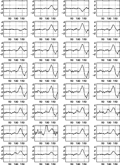
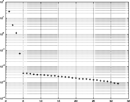
Statistical preprocessing of the data     Figure: Simulated scalp potentials due to three dipole sources mapped onto 32 channels (electrodes). Channels are numbered left to right, top to bottom. The first channel is the reference electrode. These signals are the input data for the ICA algorithm. The locations of these 32 electrodes are shown in Fig. 3.     Figure 7: Singular values of the covariance matrix. It appears that only the first four singular values contribute to the signal subspace, with the rest constituting the noise subspace. In EEG experiments, electric potential is measured with an array of electrodes (typically 32, 64, or 128) positioned primarily on the top half of the head, as shown in Fig. 3. The data are typically sampled every millisecond during an interval of interest. For a given electrode configuration, the time-dependent data can be arranged as a matrix, where every column corresponds to the sampled time frame and every row corresponds to a channel (electrode). For example, the data obtained by 32 electrodes in 180 ms can be sampled in 180 frames and represented as a matrix (32  180). Below we will refer to this matrix as  , where instead of a continuous variable t, we have sampled time frames  . Before performing source localization, we will preprocess the EEG activation maps in order to decompose them into several independent activation maps. The source for each activation map will then be localized independently. This is accomplished as follows: - First, we will process the raw signals,  , in order to reduce the dimensionality of the data, and to remove some of its noise. The projection of the data on the signal subspace will be referred to as  . - The signal subspace,  , will then be decomposed into statistically independent terms,  . - Each independent activation,  , will be assumed to be due to a single stationary dipole, which we will then localize using a parameterized search algorithm. As outlined above, the first step in processing the raw EEG data,  , is to decompose the data into signal and noise subspaces by applying the Principal Component Analysis (PCA) method [30] (in the signal processing literature it is also known as the Karhunen-Loeve transform). The decomposition is achieved by finding the eigendecomposition of the data covariance matrix: and constructing signal and noise subspaces [15]. The noise subspace will constitute the singular vectors with singular values less than a chosen noise threshold. Having constructed the subspaces, we can project the original data onto the signal subspace by:    where  and  are the signal subspace singular values and singular vectors. Though PCA allows us to estimate the number of dipoles, in the presence of noise it does not necessarily give an accurate result [15]. In order to separate out any remaining noise, as well as each statistically independent term, we will use the recently derived infomax technique, Independent Component Analysis (ICA). (It is worth noting that PCA not only filters out noise from the data, but also makes a preliminary step of ICA decomposition by decorrelating the channels, or removing linear dependence, i.e.,  . ICA then makes the channels independent, i.e.,  for any powers n and m.) There are several assumptions one needs to make about the sources in order to apply the ICA algorithm in electroencephalography [19]: - the sources must be independent (signals come from statistically independent brain processes); - there is no delay in signal propagation from the sources to the detectors (conducting media without delays at source frequencies); - the mixture is linear (Poisson's equation is linear); - the number of independent signal sources does not exceed the number of electrodes (we expect to have fewer strong sources than our 32 electrodes). It follows then that since the PCA-processed EEG recordings  are the result of linear combinations of the source signals  , they can therefore be expressed as: where  is the so-called ``mixing'' matrix and each row of  is a source's time activation. What we would like to find is an ``unmixing'' matrix  , such that: or, in other words,  ; but we do not know M, the only data we have is the  matrix. Under the assumption of independent sources, ICA allows us to construct such a  matrix; however, since neither the matrix nor the sources are known,  can be restored only up to scaling and permutations (i.e.,  is not an identity matrix, but rather is equal to  , where  is a diagonal scaling matrix and  is a permutation matrix). This problem is often referred to as Blind Source Separation (BSS) [18, 31, 32, 33].     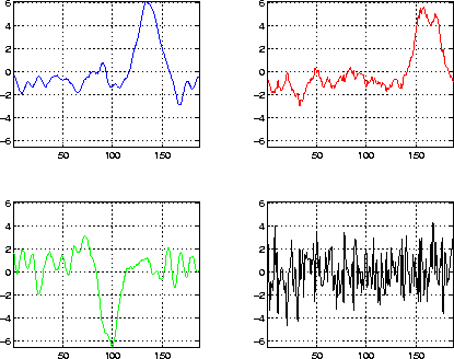Figure 8: ICA activation maps obtained by unmixing the signals from the signal subspace. We observe that there are only three independent patterns, indicating the presence of only three separate signals in the original data; the fourth component is noise. The ICA process consists of two phases: the learning phase and the processing phase. During the learning phase, the ICA algorithm finds a weighting matrix  , which minimizes the mutual information between channels (variables), i.e., makes output signals that are statistically independent in the sense that the multivariate probability density function of the input signals becomes equal to the product of  probability density functions (p.d.f.) of every independent variable. This is equivalent to maximizing the entropy of a non-linearly transformed vector  :    where  is some non-linear function. There exist several different ways to estimate the W matrix. For example, the Bell-Sejnowski infomax algorithm [18] uses weights that are changed according to the entropy gradient. Below, we use a modification of this rule as proposed by Amari, Cichocki and Yang [20], which uses the natural gradient rather than the absolute gradient of  . This allows us to avoid computing matrix inverses and to speed up solution convergence: where the vector  is defined as: and for the nonlinear function g we used: In the above equation  is a learning rate and  is the identity matrix [33]. The learning rate decreases during the iterations and we stop when  becomes smaller than a pre-defined tolerance (e.g.,  ).     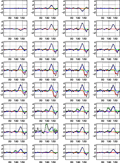Figure: The projection of the first three activation maps from Fig. 8 (as well as the original signals from Fig. 7) onto the 32 electrodes. The second phase of the ICA algorithm is the actual source separation. Independent components (activations) can be computed by applying the unmixing matrix  to the signal subspace data:    Projection of independent activation maps  back onto the electrodes one at a time can be done by: where  is the set of scalp potentials due to just the  source. For  we zero out all rows but the  ; that is, all but the  source are ``turned off''. In practice we will not need the full time sequence  in order to localize source  , but rather simply a single instant of activation. For this purpose, we set the  terms to be unit sources (i.e.,  ), resulting in  row elements which are simply the corresponding columns of  .           Fri Oct 8 13:55:47 MDT 1999

 
Revised: March , 2005