Next: Fiber Tracing Algorithm
Up: Method
Previous: Streamline Integration
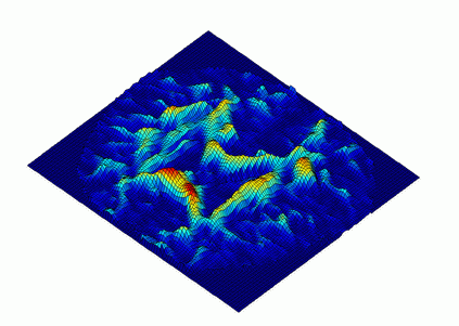
Figure 6:
Height plot for anisotropy measure (``mountain'' function) described in Section 2.6 for an axial slice of the data. The higher portions, red, corresponds to stronger anisotropy. See Eq.
 .
.
For the continuous tensor field, we use a anisotropy measure height
function
 , defined using a continues version of Eq. 4:
 |
(30) |
where  are eigenvalues of
 .
Metaphorically, we call this a ``mountain function'' because we
initiate the fibers at the high points and peaks of the mountain (the
most highly directional portions of a region) and grow them following
the major eigenvector directions. The metaphor continues as the
anisotropy measure decreases; we let the fibers grow until they go
``under water'' into the lakes (corresponding to a chosen lower value
for the anisotropy measure); the low anisotropy values indicate an
absence of fibers.
We can also incorporate the mountain function within the filter function
 itself, so that the higher regions will be given more weight in the
scheme.
Next: Fiber Tracing Algorithm
Up: Method
Previous: Streamline Integration
Leonid Zhukov
2003-01-05

![]() , defined using a continues version of Eq. 4:
, defined using a continues version of Eq. 4: