Next: Algorithm
Up: Method
Previous: Method
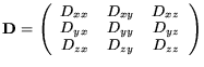
Diffusion tensors describe the diffusion properties of the media, that is
the ability of water molecules to move around. In biological tissues
diffusion properties are dictated by the cell structure of the
tissue. Water molecules can easily move inside the cell, but their
motion across the cells is restricted by the cell membrane. Thus diffusion
properties of the tissue reflect the shape and orientation of the cells.
In the case of an elongated cell, the tissue will have a
preferred diffusion direction along the primary axis of the cell.
Diffusion is measured through a diffusion coefficient, which
is represented with a symmetric second order tensor -
 x matrix:
|
 |
|
|
(1) |
The  independent values (the tensor is symmetric) of the tensor
elements vary continuously with the spatial location in the tissue.
Eigenvalues
independent values (the tensor is symmetric) of the tensor
elements vary continuously with the spatial location in the tissue.
Eigenvalues  and eigenvectors
 of a matrix
(1) can be found as a solution to the eigenvalue problem:
of a matrix
(1) can be found as a solution to the eigenvalue problem:
 |
(2) |
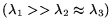
Since the tensor is symmetric, its eigenvalues are always real
numbers, and the eigenvectors are orthogonal and form a basis.
Geometrically, a diffusion tensor can be thought of as an ellipsoid
with its three axes oriented along these eigenvectors, with the three
semi-axis lengths proportional to the square root of the eigenvalues
of the tensor - mean diffusion distances [Basser et al. 1994].
Using the ellipsoidal interpretation, one can classify the diffusion
properties of a tissue according to the shape of the ellipsoids, with
extended ellipsoids corresponding to regions with strong linear
diffusion (long, thin cells), flat ellipsoids to planar diffusion, and
spherical ellipsoids to regions of isotropic media (such as
fluid-filled regions like the ventricles). The quantitative
classification can be done through the coefficients
 [Westin et al. 1997] corresponding to linear, planar and spherical diffusion.
These coefficients are normalized to the range of
![$[0..1]$](img14.gif) . Values of
. Values of
 that are close to
 selects regions with strong linear
 diffusion. Values of
 and
and  will be small in those regions. Large
values
correspond to planar diffusion, large
values corresponds to
isotropic media.
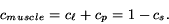
Due to the structure of the heart muscle, we will use the sum of the
and
coefficients to characterize the tissue, thus looking for regions with high
combined directional and planar anisotropies
will be small in those regions. Large
values
correspond to planar diffusion, large
values corresponds to
isotropic media.
Due to the structure of the heart muscle, we will use the sum of the
and
coefficients to characterize the tissue, thus looking for regions with high
combined directional and planar anisotropies
 |
(4) |
This approach retains all of the directional information from
 and and discards all
nondirectional .
and and discards all
nondirectional .
Next: Algorithm
Up: Method
Previous: Method
Leonid Zhukov
2003-09-10